Structure from Motion
This article is written by Chahat Deep Singh.
Table of Contents:
- Introduction
- Feature Matching
- Estimating Fundamental Matrix
- Estimate Camera Pose from Essential Matrix
- Check for Cheirality Condition using Triangulation
- Bundle Adjustment
- Summary
Introduction
We have been playing with images for so long, mostly in 2D scene. Recall project 2 where we stitched multiple images with about 30-50% common features between a couple of images. Now let’s learn how to reconstruct a 3D scene and simultaneously obtain the camera poses of a monocular camera w.r.t. the given scene. This procedure is known as Structure from Motion (SfM). As the name suggests, you are creating the entire rigid structure from a set of images with different view points (or equivalently a camera in motion). A few years ago, Agarwal et. al published Building Rome in a Day in which they reconstructed the entire city just by using a large collection of photos from the Internet. Ever heard of Microsoft Photosynth? Facinating? isn’t it!? There are a few open source SfM algorithm available online like VisualSFM. Try them!
Let’s learn how to recreate such algorithm. There are a few steps that collectively form SfM:
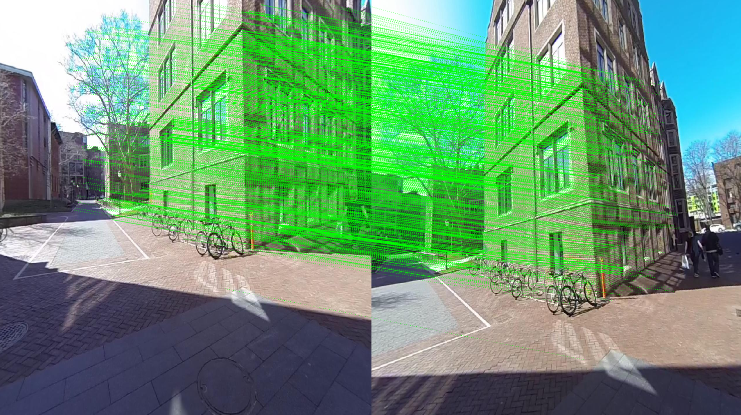
- Feature Matching and Outlier rejection using RANSAC
- Estimating Fundamental Matrix
- Estimating Essential Matrix from Fundamental Matrix
- Estimate Camera Pose from Essential Matrix
- Check for Cheirality Condition using Triangulation
- Perspective-n-Point
- Bundle Adjustment
(If you haven’t heard of the above terminology before, don’t worry! If you knew the following already, you wouldn’t be taking the class right now!)
1. Feature Matching, Fundamental Matrix and RANSAC:
We have already learned about keypoint matching using SIFT keypoints and descriptors (Recall Project 2: Panorama Stitching). It is important to refine the matches by rejecting outline correspondence. Before rejecting the correspondences, let us first understand what Fundamental matrix is!
1.1. Estimating Fundamental Matrix:
The fundamental matrix, denoted by \(F\), is a \(3\times 3\) (rank 2) matrix that relates the corresponding set of points in two images from different views (or stereo images). But in order to understand what fundamental matrix actually is, we need to understand what epipolar geometry is! The epipolar geometry is the intrinsic projective geometry between two views. It only depends on the cameras’ internal parameters (\(K\) matrix) and the relative pose i.e. it is independent of the scene structure.
1.2. Epipolar Geometry:
Let’s say a point \(\mathbf{X}\) in the 3D-space (viewed in two images) is captured as \(\mathbf{x}\) in the first image and \(\mathbf{x'}\) in the second. Can you think how to formulate the relation between the corresponding image points \(\mathbf{x}\) and \(\mathbf{x'}\)? Consider Fig. 2. Let \(\mathbf{C}\) and \(\mathbf{C'}\) be the respective camera centers which forms the baseline for the stereo system. Clearly, the points \(\mathbf{x}\), \(\mathbf{x'}\) and \(\mathbf{X}\) (or \(\mathbf{C}\), \(\mathbf{C'}\) and \(\mathbf{X}\)) are coplanar i.e. \(\mathbf{\overrightarrow{Cx}}\cdot \left(\mathbf{\overrightarrow{CC'}}\times\mathbf{\overrightarrow{C'x'}}\right)=0\) and the plane formed can be denoted by \(\pi\). Since these points are coplanar, the rays back-projected from \(\mathbf{x}\) and \(\mathbf{x'}\) intersect at \(\mathbf{X}\). This is the most significant property in searching for a correspondence.
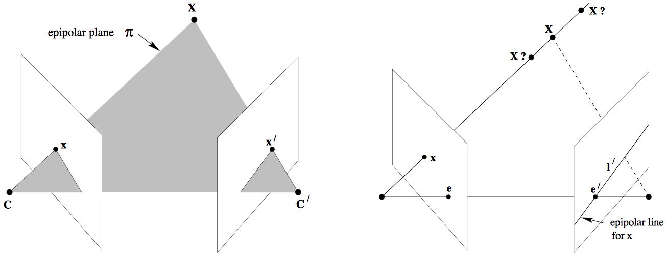
Now, let us say that only \(\mathbf{x}\) is known, not \(\mathbf{x'}\). We know that the point \(\mathbf{x'}\) lies in the plane \(\pi\) which is governed by the camera baseline \(\mathbf{CC'}\) and \(\mathbf{\overrightarrow{Cx}}\). Hence the point \(\mathbf{x'}\) lies on the line of intersetion of \(\mathbf{l'}\) of \(\pi\) with the second image plane. The line \(\mathbf{l'}\) is the image in the second view of the ray back-projected from \(\mathbf{x}\). This line \(\mathbf{l'}\) is called the epipolar line corresponding to \(\mathbf{x}\). The benifit is that you don’t need to search for the point corresponding to \(\mathbf{x}\) in the entire image plane as it can be restricted to the \(\mathbf{l'}\).
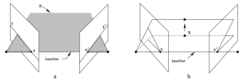
- Epipole is the point of intersection of the line joining the camera centers with the image plane. (see \(\mathbf{e}\) and \(\mathbf{e'}\) in the Fig. 2(a))
- Epipolar plane is the plane containing the baseline.
- Epipolar line is the intersection of an epipolar plane with the image plane. All the epipolar lines intersect at the epipole.
1.3 The Fundamental Matrix \(\mathbf{F}\):
The \(\mathbf{F}\) matrix is only an algebraic representation of epipolar geometry and can both geometrically (contructing the epipolar line) and arithematically. (See derivation) (Fundamental Matrix Song) As a result, we obtain: \(\mathbf{x}_i'^{\ \mathbf{T}}\mathbf{F} \mathbf{x}_i = 0\) where \(i=1,2,....,m.\) This is known as epipolar constraint or correspondance condition (or Longuet-Higgins equation). Since, \(\mathbf{F}\) is a \(3\times3\) matrix, we can set up a homogenrous linear system with 9 unknowns:
\[\begin{bmatrix} x'_i & y'_i & 1 \end{bmatrix} \begin{bmatrix}f_{11} & f_{12} & f_{13} \\ f_{21} & f_{22} & f_{23} \\ f_{31} & f_{32} & f_{33} \end{bmatrix} \begin{bmatrix} x_i \\ y_i \\ 1 \end{bmatrix} = 0\]\(\begin{equation}x_i x'_i f_{11} + x_i y'_i f_{21} + x_i f_{31} + y_i x'_i f_{12} + y_i y'_i f_{22} + y_i f_{32} + x'_i f_{13} + y'_i f_{23} + f_{33}=0\end{equation}\)
Simplifying for \(m\) correspondences,
\[\begin{bmatrix} x_1 x'_1 & x_1 y'_1 & x_1 & y_1 x'_1 & y_1 y'_1 & y_1 & x'_1 & y'_1 & 1 \\ \vdots & \vdots & \vdots & \vdots & \vdots & \vdots & \vdots & \vdots & \vdots \\ x_m x'_m & x_m y'_m & x_m & y_m x'_m & y_m y'_m & y_m & x'_m & y'_m & 1 \end{bmatrix}\begin{bmatrix} f_{11} \\ f_{21} \\ f_{31} \\ f_{12} \\ f_{22} \\ f_{32} \\ f_{13} \\f_{23} \\ f_{33}\end{bmatrix} = 0\]How many points do we need to solve the above equation? Think! Twice! Remember homography, where each point correspondence contributes two constraints? Unlike homography, in \(\mathbf{F}\) matrix estimation, each point only contributes one constraints as the epipolar constraint is a scalar equation. Thus, we require at least 8 points to solve the above homogenous system. That is why it is known as Eight-point algorithm.
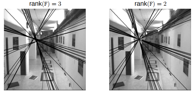
With \(N \geq 8\) correspondences between two images, the fundamental matrix, \(F\) can be obtained as: By stacking the above equation in a matrix \(A\), the equation \(Ax=0\) is obtained. This system of equation can be answered by solving the linear least squares using Singular Value Decomposition (SVD) as explained in the Math module. When applying SVD to matrix \(\mathbf{A}\), the decomposition \(\mathbf{USV^T}\) would be obtained with \(\mathbf{U}\) and \(\mathbf{V}\) orthonormal matrices and a diagonal matrix \(\mathbf{S}\) that contains the singular values. The singular values \(\sigma_i\) where \(i\in[1,9], i\in\mathbb{Z}\), are positive and are in decreasing order with \(\sigma_9=0\) since we have 8 equations for 9 unknowns. Thus, the last column of \(\mathbf{V}\) is the true solution given that \(\sigma_i\neq 0 \ \forall i\in[1,8], i\in\mathbb{Z}\). However, due to noise in the correspondences, the estimated \(\mathbf{F}\) matrix can be of rank 3 i.e. \(\sigma_9\neq0\). So, to enfore the rank 2 constraint, the last singular value of the estimated \(\mathbf{F}\) must be set to zero. If \(F\) has a full rank then it will have an empty null-space i.e. it won’t have any point that is on entire set of lines. Thus, there wouldn’t be any epipoles. See Fig. 3 for full rank comparisons for \(F\) matrices.
In MATLAB, you can use svd to solve \(\mathbf{x}\) from \(\mathbf{Ax}=0\)
[U, S, V] = svd(A);
x = V(:, end);
F = reshape(x, [3,3])';
1.4. Match Outlier Rejection via RANSAC:
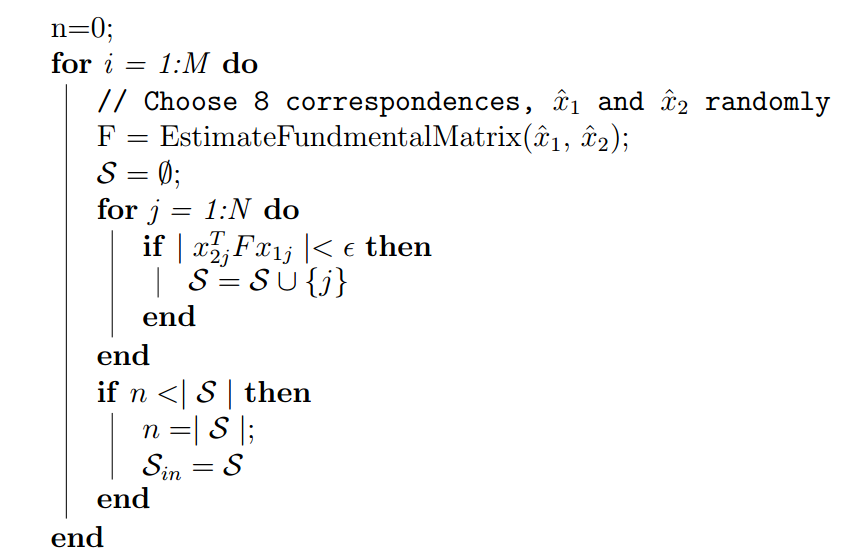
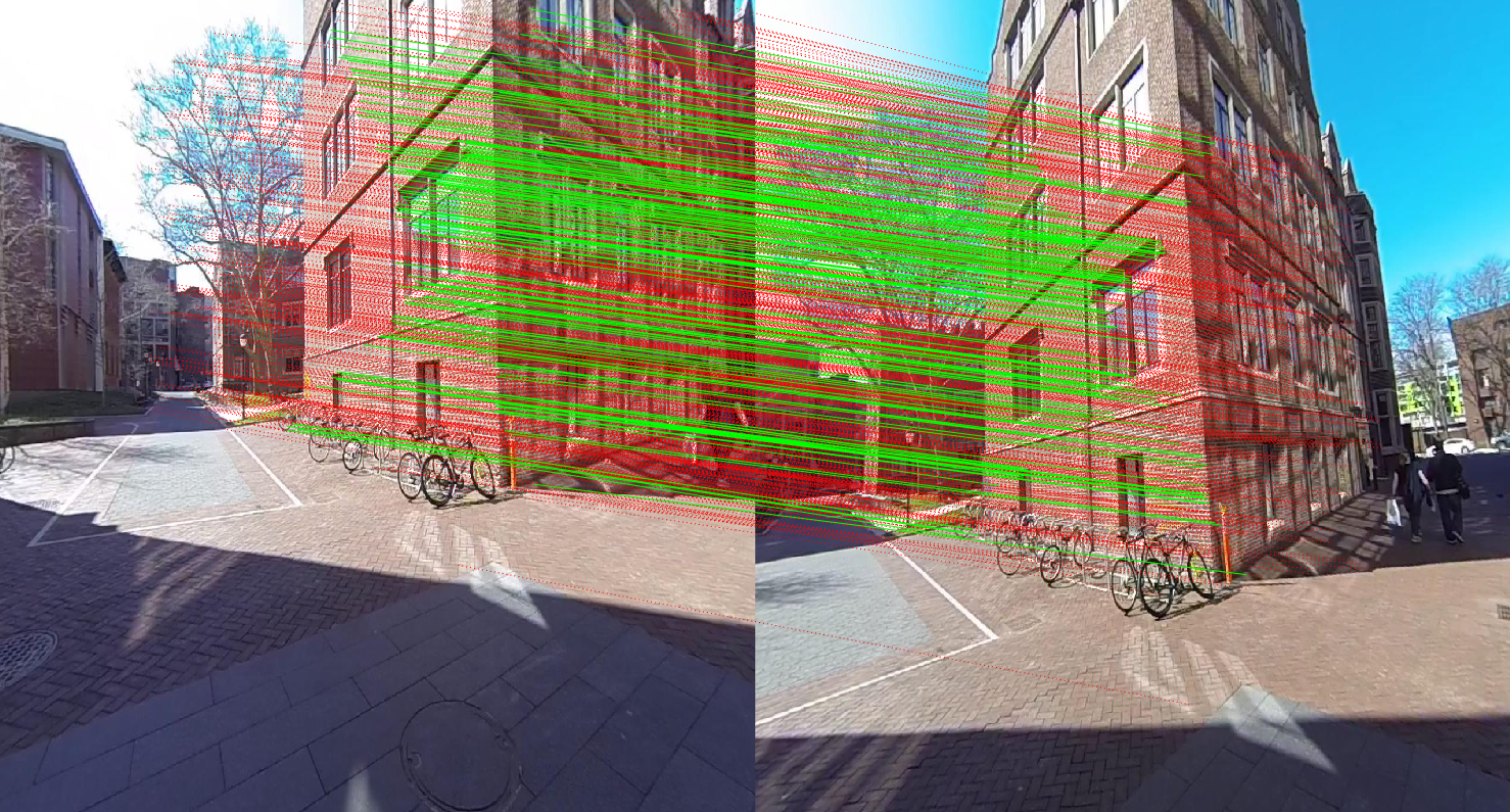
Since the point correspondences are computed using SIFT or some other feature descriptors, the data is bound to be noisy and (in general) contains several outliers. Thus, to remove these outliers, we use RANSAC algorithm (Yes! The same as used in Panorama stitching!) to obtain a better estimate of the fundamental matrix. So, out of all possibilities, the \(\mathbf{F}\) matrix with maximum number of inliers is chosen. Below is the pseduo-code that returns the \(\mathbf{F}\) matrix for a set of matching corresponding points (computed using SIFT) which maximizes the number of inliers.
2. Estimate Essential Matrix from Fundamental Matrix:
Since we have computed the \(\mathbf{F}\) using epipolar constrains, we can find the relative camera poses between the two images. This can be computed using the Essential Matrix, \(\mathbf{E}\). Essential matrix is another \(3\times3\) matrix, but with some additional properties that relates the corresponding points assuming that the cameras obeys the pinhole model (unlike \(\mathbf{F}\)). More specifically, \(\mathbf{E}\) = \(\mathbf{K^TFK}\) where \(\mathbf{K}\) is the camera calibration matrix or camera intrinsic matrix. Clearly, the essential matrix can be extracted from \(\mathbf{F}\) and \(\mathbf{K}\). As in the case of \(\mathbf{F}\) matrix computation, the singular values of \(\mathbf{E}\) are not necessarily \((1,1,0)\) due to the noise in \(\mathbf{K}\). This can be corrected by reconstructing it with \((1,1,0)\) singular values, i.e. \(\mathbf{E}=U\begin{bmatrix}1 & 0 & 0 \\ 0 & 1 & 0 \\ 0 & 0 & 0 \end{bmatrix}V^T\)
It is important to note that the \(\mathbf{F}\) is defined in the original image space (i.e. pixel coordinates) whereas \(\mathbf{E}\) is in the normalized image coordinates. Normalized image coordinates have the origin at the optical center of the image. Also, relative camera poses between two views can be computed using \(\mathbf{E}\) matrix. Moreover, \(\mathbf{F}\) has 7 degrees of freedom while \(\mathbf{E}\) has 5 as it takes camera parameters in account. (5-Point Motion Estimation Made Easy)
3. Estimate Camera Pose from Essential Matrix
The camera pose consists of 6 degrees-of-freedom (DOF) Rotation (Roll, Pitch, Yaw) and Translation (X, Y, Z) of the camera with respect to the world. Since the \(\mathbf{E}\) matrix is identified, the four camera pose configurations: \((C_1, R_1), (C_2, R_2), (C_3, R_3)\) and \((C_4, R4)\) where \(\ C\in\mathbb{R}^3\) is the camera center and \(R\in SO(3)\) is the rotation matrix, can be computed. Thus, the camera pose can be written as: \(P = KR\begin{bmatrix}I_{3\times3} & -C\end{bmatrix}\) These four pose configurations can be computed from \(\mathbf{E}\) matrix. Let \(\mathbf{E}=UDV^T\) and \(W=\begin{bmatrix}0 & -1 & 0\\ 1 & 0 & 0\\ 0 & 0 & 1\end{bmatrix}\). The four configurations can be written as:
- \(C_1=U(:, 3)\) and \(R_1=UWV^T\)
- \(C_2=-U(:, 3)\) and \(R_2=UWV^T\)
- \(C_3=U(:, 3)\) and \(R_3=UW^TV^T\)
- \(C_4=-U(:, 3)\) and \(R_4=UW^TV^T\)
It is important to note that the \(\ det(R)=1\). If \(det(R)=-1\), the camera pose must be corrected i.e. \(C=-C\) and \(R=-R\).
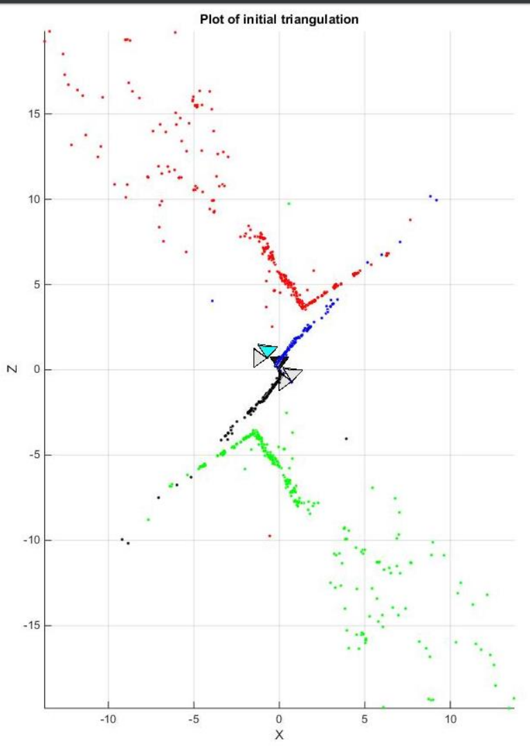
4. Check for Cheirality Condition using Triangulation:
In the previous section, we computed four different possible camera poses for a pair of images using essential matrix. Though, in order to find the correct unique camera pose, we need to remove the disambiguity. This can be accomplish by checking the cheirality condition i.e. the reconstructed points must be in front of the cameras. To check the cheirality condition, triangulate the 3D points (given two camera poses) using linear least squares to check the sign of the depth \(Z\) in the camera coordinate system w.r.t. camera center. A 3D point \(X\) is in front of the camera iff: \(r_3\mathbf{(X-C)} > 0\) where \(r_3\) is the third row of the rotation matrix (z-axis of the camera). Not all triangulated points satisfy this coniditon due of the presence of correspondence noise. The best camera configuration, \((C, R, X)\) is the one that produces the maximum number of points satisfying the cheirality condition.
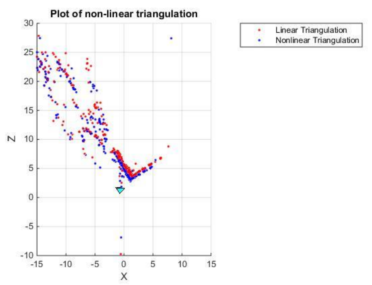
4.1 Non-Linear Triangulation:
Given two camera poses and linearly triangulated points, \(X\), the locations of the 3D points that minimizes the reprojection error (Recall Project 2) can be refined. The linear triangulation minimizes the algebraic error. Though, the reprojection error is geometrically meaningful error and can be computed by measuring error between measurement and projected 3D point:
\(\underset{x}{\operatorname{min}}\) \(\sum_{j=1,2}\left(u^j - \frac{P_1^{jT}\widetilde{\phi}}{P_3^{jT}{X}}\right)^2 + \left(v^j - \frac{P_2^{jT}\widetilde{\phi}}{P_3^{jT}{X}}\right)^2\)
Here, \(j\) is the index of each camera, \(\widetilde{X}\) is the hoomogeneous representation of \(X\). \(P_i^T\) is each row of camera projection matrix, \(P\). This minimization is highly nonlinear due to the divisions. The initial guess of the solution, \(X_0\), is estimated via the linear triangulation to minimize the cost function. This minimization can be solved using nonlinear optimization toolbox such as fminunc or lsqnonlin in MATLAB.
5. Perspective-\(n\)-Points:
Now, since we have a set of \(n\) 3D points in the world, their \(2D\) projections in the image and the intrinsic parameter; the 6 DOF camera pose can be estimated using linear least squares. This fundamental problem, in general is known as Persepective-\(n\)-Point (PnP). For there to exist a solution, \(n\geq 3\). There are multiple methods to solve the P\(n\)P problem and have an assumptions in most of them that the camera is calibrated. Methods such as Unified P\(n\)P (or UPnP) do not abide with the said assumption as they estimate both intrinsic and extrinsic parameters.
P\(n\)P is prone to error as there are outliers in the given set of point correspondences. To overcome this error, we can use RANSAC (yes, again!) to make our camera pose more robust to outliers. The alogrithm below depicts the solution with RANSAC.
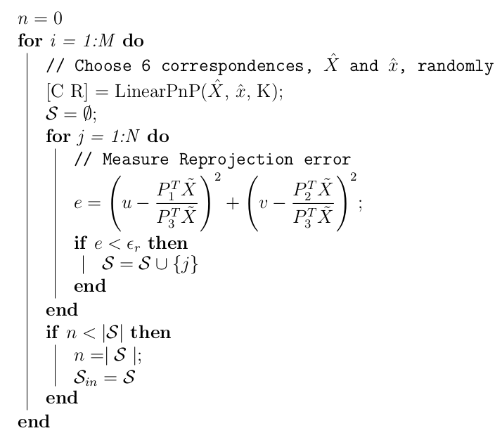
Just like in triangulation, since we have the linearly estimated camera pose, we can refine the camera pose that minimizes the reprojection error (Linear PnP only minimizes the algebraic error). Though, reprojection error is the geometrically meaningful error and can be computed by measuring error between measurement and projected 3D point.
\(\underset{C,R}{\operatorname{min}} \sum_{i=1,J} \left(u^j - \frac{P_1^{jT}\widetilde{X_j}}{P_3^{jT}{\widetilde{X_j}}}\right)^2 + \left(v^j - \frac{P_2^{jT}\widetilde{X_j}}{P_3^{jT}{X_j}}\right)^2\)
6. Bundle Adjustment:
Once you have computed all the camera poses and 3D points, we need to refine the poses and 3D points together, initialized by previous reconstruction by minimizing reporjection error.
The optimization problem can formulated as following:
\(\underset{\{C_i, q_i\}_{i=1}^i,\{X\}_{j=1}^J}{\operatorname{min}}\sum_{i=1}^I\sum_{j=1}^J V_{ij}\left(\left(u^j - \dfrac{P_1^{jT}\tilde{\phi}}{P_3^{jT}\tilde{X}}\right)^2 + \left(v^j - \dfrac{P_2^{jT}\tilde{\phi}}{P_3^{jT}\tilde{X}}\right)^2\right)\) where \(V_{ij}\) is the visibility matrix. (Don’t scratch your head yet!)
Visibility matrix signifies the relationship between the camera and a point. \(V_{ij}\) is one if \(j^{th}\) point is visible from the \(i^{th}\) camera and zero otherwise. One can use a nonlinear optimization toolbox such as fminunc or lsqnonlin in MATLAB but is extremely slow as the number of parameters are large. The Sparse Bundle Adjustment toolbox is designed to solve such optimization problem by exploiting sparsity of visibility matrix, \(V\).
Clearly, solving such a method to compute the structure from motion is complex and slow (can take upto an hour for only 8-10 images). The above steps collectively is the traditional way of solving the problem of SfM. However, due to recent advances in graph optimization for visual systems, we can solve the same problem in real time. Let’s read further about the modern approach of solving the same problem.