Rotobrush
This article is written by Chahat Deep Singh.
Table of Content:
- Introduction
- Overview
- Segmenting Localized Classifiers
- Updating Window Locations
- Update Local Classifier
- Updating the Shape and Color Models
- Merging Local Windows
- References
1. Introduction
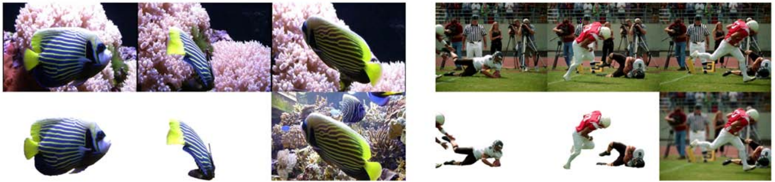
In this project, we will learn segmenting objects in a video sequence. Given a good boundary detection in the initial frame of a video, the object can be tracked and segmented out in the remaining sequence. It is much easier to segment the rigid objects in the scene using traditional tracking algorithms but the same can’t be said for deformable objects like the one you can see in the Fig. 1.
In this article, we specifically will implement an algorithm called Video SnapCut (also known as RotoBrush in Adobe After Effects) by Bai et. al. To get a very good inituition, we would highly recommend watching this 5 min video that describes the entire paper.
Note: Reading the paper [1] is HIGHLY RECOMMENDED.
2. Overview
As mentioned in the introduction section, we need to provide a foreground mask for the object that needs to be segmented. This can be done using roipoly from Image Processing Toolbox in MATLAB. The SnapCut can then sample a series of overlapping image windows along the object’s boundary. For each such windows, a local classifier is created which is trained to classify whether a pixel belongs to foreground or background. The classifier is trained in such a way that it not only takes into account the color (like [2]) but shape as well.
For the subsequent frames, the local classifiers are used for estimating an updated foreground mask. First, the object’s movements between frames is estimated for reposition of the image windows. The goal is to have the windows stay in the same position on the object’s boundary, or the most similar place possible. With the window positions updated, we then use the local classifiers to re-estimate the foreground mask for each window. These windows overlap, so we merge their foreground masks together to obtain a final, full-object mask. Optionally, we can rerun the local classifiers and merging steps to refine the mask for this frame. Before moving on to the next frame, we re-train the local classifiers, so they remain accurate despite changes in background (and possibly foreground) appearance.
NOTE:
In order to develop a practical video cutout that can perform on complicated video with deformable objects, it is import to follow the two underlying principles:
1. Multiple cues should be used for extracting the foreground such as color, shape, motion and texture information. Among these, shape plays a vital role for maintaining a temporally-coherent recognition.
2. Multiple cues should be evaluated and integrated not just globally, but locally as well in order to maximize their discriminant powers.
3. Segmenting with Localized Classifiers
3.1. Local Windows
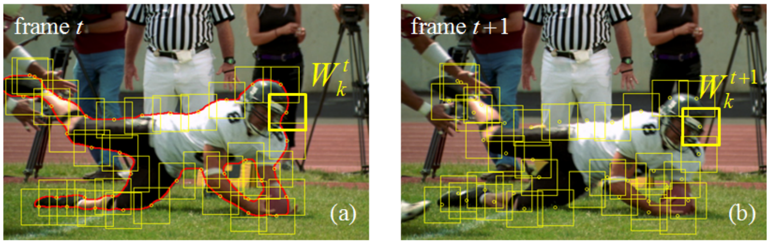
Once the initial mask is obtained, say \(L^t(x)\) on a keyframe \(I_t\), a set of overlapping windows \(W_q^t,...,W_n^t\) along its contour \(C_t\) are to be uniformly sampled as shown in Fig. 3. Assume single contour for now, multiple contours can be handled in the same way. The size and density of the windows can be chosen emperically, usually \(30\times30\) to \(80\times80\) pixels. Each window defines the application range of a local classifier, and the classifier will assign to every pixel inside the window a foreground (object) probability, based on the local statistics it gathers. Neighboring windows overlap for about one-third of the window size.
Note: Since each local window moves along its own (averaged) motion vector, the distances between updated neighboring windows may slightly vary. This is one of the main reasons to use overlapping windows in the keyframe, so that after propagation, the foreground boundary is still fully covered by the windows.
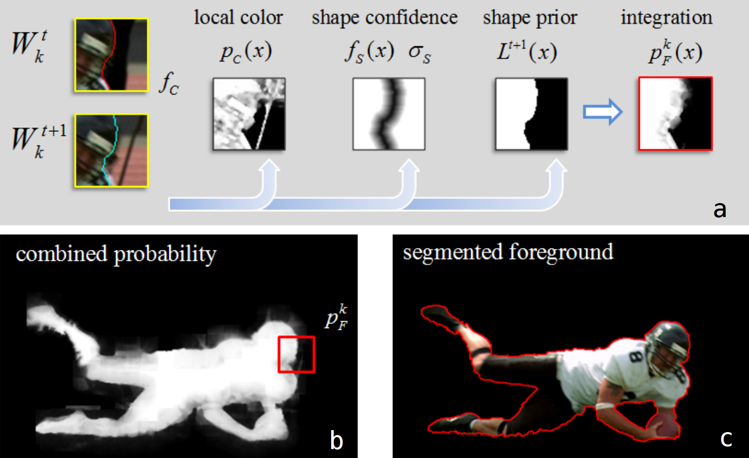
The window-level local classifiers are composed of a color model (GMM), a shape model (the foreground mask and a shape confidence mask). Confidence metrics are calculated for the color and shape models: for the color model this is a single value, and for the shape model it is a mask. When the color and shape models are integrated into a single mask, the confidence values are used to assign more weight to the more confident model. Fig. 4 illustrates the segmented foreground and combined probability for local classifiers.
3.2. Initializing the Color Model
The purpose of the color model is to classify pixels as foreground \(\mathcal{F}\) or background \(\mathcal{B}\) based on their color. The assumption is that \(\mathcal{F}\) and \(\mathcal{B}\) pixels generally differ in color. The color model is based on GMM. One can use Matlab’s fitgmdist and gmdistribution function from Statistics and Machine Learning toolbox.
In order to create the color model, two GMMs are build for \(\mathcal{F}\) and \(\mathcal{B}\) regions seperately.
Note: Use Lab color space for the color models. To avoid possible sampling errors, we only use pixels whose spatial distance to the segmented boundary is larger than a threshold (5 pixels in our system) as the training data for the GMMs.
Now, for a pixel \(x\) in the window, its foreground probability generated from the color model is computed as:
\[p_c(x)=p_c(x \vert \mathcal{F})\ / \ \left(p_c(x \vert \mathcal{F})+p_c(x \vert \mathcal{B})\right)\]where \(p_c\), \(p_c(x \vert \mathcal{F})\) and \(p_c(x \vert \mathcal{B})\) are the corresponding probabilities computed from the two GMMs. Refer to section 2.1 for more details.
3.3. Color Model Confidence
The local color model confidence \(f_c\) is used to describe how separable the local foreground is against the local background using just the color model. Let \(L^t(x)\) be the known segmentation label (\(\mathcal{F}=1\) and \(\mathcal{B}=0)\) of pixel \(x\) for the current frame, \(f_c\) is computed as
\[f_c=1-\cfrac{\int_{W_k}|L^t(x)-p_c(x)|\cdot\omega_c(x)dx}{\int_{W_k}\omega_c(x)dx}\]The weighing function \(\omega_c(x)\) is computed as \(\omega_c(x)=exp(-d^2(x)\ /\ \sigma_c^2\), where \(d(x)\) is the spatial distance between \(x\) and the foreground boundary, computed using the distance transform. \(\sigma_c\) is fixed as half of the window size. \(\omega_c(x)\) is higher when \(x\) is closer to the boundary i.e. the color model is required to work well near the foreground boundary for accurate segmentation.
3.4. Shape Model
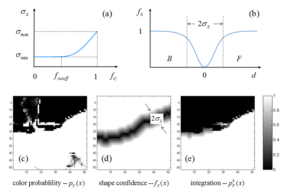
The local shape model \(M_s\) contains the existing segmentation mask \(L^t(x)\) and a shape confidence mask computed as
\[f_s(x)=1-exp(-d^2(x)\ /\ \sigma^2_s)\]where \(d(x)\) stands for the distance to the foreground boundary and \(\sigma_s\) is a parameter. A larger \(\sigma_s\) means the shape confidence is low around the foreground boundary while a small \(\sigma_s\) means high confidence on the segmentation mask \(L^t(x)\). Fig. 5(d) shows an example of the shape confidence map. Note: \(\sigma_s\) is a very important parameter in this approach and can be adaptively and automatically adjusted to achieve accurate local segmentation. A simple explanation for updating local models can be found in section 2.3 in [1].
4. Updating Window Locations
In the previous section, we set up local classifiers for identifying foreground and background pixels within their windows. As we move on to the next video frame, the object and background may move and/or change. Our local classifier windows must move to stay centered on approximately the same place on the object’s boundary. We accomplish this by tracking two kinds of motion: the rigid motion of the whole object, and then the smaller local deformations of the object’s boundary. For example, in Fig. 3, the football player is overall falling downwards (motion affecting the entire object), as well as bending his arms, turning his head, bending his legs, etc. (changing specific regions of the object’s boundary).
4.1. Estimate the Motion of the Entire Object
To estimate the overall motion of the object, find matching feature points on the object in the two frames, and use them to find an affine transform between the images. Use this to align the object in frame 1 to frame 2. “This initial shape alignment usually captures and compensates for large rigid motions of the foreground object.” Use Matlab’s estimateGeometricTransform to do so.
4.2. Estimate Local Boundary Deformation
After applying the affine transform from the previous step, we want to track the boundary movement/deformation for the local windows. Optical flow will give us an estimate of each pixel’s motion between frames. However, “optical flow is unreliable, especially near boundaries where occlusions occur” [1]. Luckily, we know exactly where the object’s boundary is! Thus, to get a more accurate estimate, find the average of the flow vectors inside the object’s bounds. Use this average vector to estimate how to re-center the local window in the new frame.
While this method for window re-positioning is not perfect, errors are accommodated by the significant overlap between neighboring windows: they should still overlap enough that the object’s entire boundary is covered. You can use Matlab’s optical flow functionality, such as the opticalFlowHS function.
5. Update Local Classifier
Now that the local windows have been properly re-centered, we can update the local classifiers for the new frame.
5.1. Updating the Shape Model
The shape model is composed of the foreground mask and the shape confidence map. These are both carried over from the previous frame.
5.2. Updating the Color Model
The distribution of colors in the foreground and background may change from one frame to the next, as different parts of the scene move independently. We want to update the color model to reflect these changes. Simply replacing the existing color model with a new pair of GMMs every frame could pose problems. For one, if there’s a sudden change in color in one frame, which quickly disappears in the next, our color model will be completely de-railed.
Moreover, the new GMMs may have degraded performance because of improper labling of the pixels used to train them. This is because we label “foreground” and “background” pixels based on the foreground mask, and that may be less accurate after updating window locations in the previous step.
So what can we do? Bai. et. al. propose to compare two color models: the existing one from the previous frame and a combination of the previous and new frame’s GMMs. They first observe that the colors in the foreground region don’t change much between frames, while the background region can change significantly. Therefore we’d expect the number of pixels classifier by the model as foreground to be relatively consistent between frames. If the number of foreground pixels increases under the new color model, then we should stick with the old one. If we choose the new color model, we must also re-compute the color confidence value, as was done in section 4.3.
6. Updating the Shape and Color Models
For each window, we now merge the foreground maps produced by the shape and color models, weighting them based on the shape confidence map. The foreground probability \(p_{\mathcal{F}}^k(x)\), corresponding to the window \(W_k\) in the current frame, becomes a linear combination of the updated color probability \(p_c(x)\) and the updated (warped) binary shape mask \(L^{t+1}(x)\), using the shape confidence map \(f_s(x)\) with the just computed \(\sigma_s\) as the interpolation coefficients:<
\[p_{\mathcal{F}}^k(x)=f_s(x)L^{t+1}(x)+(1-f_s(x)) \ p_c(x)\]Examples of \(p_c(x)\), \(f_s(x)\) and \(p_{\mathcal{F}}^k(x)\) are shown in Fig. 5(c,d,e).
7. Merging Local Windows
After the previous step, we have a foreground probability mask for each local window. We now merge the overlapping local windows into a global foreground mask. In this overlapping window design, a pixel is often covered by multiple adjacent windows, and its foreground probability is a weighted linear combination of the probabilities computed from each window it belongs to,
\[p_{\mathcal{F}}(x)=\cfrac{\sum_{k}p_{\mathcal{F}}^k(x)(\vert x-c_k \vert)+\epsilon)^{-1}}{\sum_k(\vert x-c_k \vert +\epsilon)^{-1}}\]where \(k\) is the index of local windows (the sum ranges over all the \(k-s\) such that the updated window \(W^{t+1}k\) covers the pixel), is a small constant (\(0.1\) in the system), and \(c_k\) is the center of the window (\(\vert x − c_k \vert\) is the distance from the pixel \(x\) to the center).
7.1. Extracting the Final Foreground Mask
This gives a real-valued probability map for the foreground mask. We want a binary mask. The simplest solution would be to threshold the values of the probability map. This may produce a somewhat rough result. Bai et. al. use Graph Cut segmentation to obtain a better final result: you are encouraged (but not required) to use Matlab’s lazysnapping tool to implement this. Fig. 6 shows the output of Video SnapCut.
SnapCut is a novel video cutout system which uses adaptive local classifiers for segmenting dynamic video objects. By localizing the classifiers, the system achieves significantly better results than other algorithms for complicated videos, including complex color distributions, dynamic backgrounds and non-rigid foreground deformations.
8. References
- Bai, X., Wang, J., Simons, D. and Sapiro, G., 2009, July. Video snapcut: robust video object cutout using localized classifiers. In ACM Transactions on Graphics (ToG) (Vol. 28, No. 3, p. 70). ACM.
- Wang, J. and Cohen, M.F., 2005, October. An iterative optimization approach for unified image segmentation and matting. In Computer Vision, 2005. ICCV 2005. Tenth IEEE International Conference on (Vol. 2, pp. 936-943). IEEE.