Structure from Motion

This article is written by Nitin J. Sanket.

Table of Contents:

• Introduction
• Detailed Explanation of Project 4

Introduction

The SfM pipeline we talked about before relies on an optimization framework to do the bundle adjustment and you would’ve also observed that we also used fminunc or lsqnonlin for solving non-linear least squares in traingulation and PnP. This is not very efficient and there has to be a better way right? Guess what, there is! In 2012, Prof. Frank Dellaert published a hallmark paper called GTSAM for solving such problems which are commonly classified as Pose Graph Optimization and uses the concept of Factor Graphs. This method has been improved over the years and has periodically improved it’s optimization methods with the latest literature. Though there are faster pose graph optimization frameworks like g2o or SLAM++, GTSAM by far is one of the easiest frameworks to setup, use and understand and hence will be the our choice to solve this project.

Let us consider a toy example to understand how one would solve SfM/SLAM in GTSAM. For the purpose of brevity, I am assuming that you have followed the setup insturctions here and setup GTSAM 3.2.1 on your computer with MATLAB compatibility. For any issues or help regarding the setup feel free to contact the TAs. Now, let’s get back to the problem in hand. The problem is defined as follows. Our robot lives in a 2D world with certain number of unique landmarks \(N\). The origin in the world and the scale is arbitrary, i.e., any point in the map can be chosen as the origin. A common choice is the start of service or the pose (position and orientation) of the robot at the beginning of the algorithm is chosen as the origin. The scale being arbitrary just means that all the distances are measured to some relative scale, i.e., metric scale is unknown. We only know that a landmark is twice as far as the other landmark and this could metrically mean that one landmark is 2m away or 2cm away, the information about this is not known. This is the case when we have only one camera. However, if a distance sensor like a SONAR or a LIDAR is used we would know the metric scale. Note that this doesn’t change anything in the algorithm or the framework but merely changes the units in the computation.

Now, let us say that each landmark is uniqely numbered so that we can distinguish between them. Let each landmark \(\mathbf{l_k}\) be represented by am \(\mathbb{R}^2\) vector which contains the \(x\) and \(y\) coordinate and is denoted by \( \mathbf{l_k} = \begin{bmatrix} l_{k,x} & _{k,y}\end{bmatrix}^T\). The SfM/SLAM problem is to find the realtive pose of the landmarks and the pose of the robot when the robot is moving in the world. The key assumption here is that the landmarks are stationary. Dealing with non-stationary objects in the world is still an unsolved research topic.

The world with numbered landmarks (red x's) and robot at time \( t = 0\) (blue circle). The start of service origin is chosen as the robot's pose at time \( t = 0\) (blue asterisk).

Mathematically, we want to get the best estimate of the landmark locations \(\mathbf{l_k}\) and robot pose at every time instant \(\mathbf{x_t}\) given the robot has a noisy sense of how it’s moving (odometry or ego-motion) denoted by \(\mathbf{o_{t}^{t+1}}\) and the noisy measurements of the some landmark location(s) at each time instant \(\mathbf{m_t}\). Let the state/pose of the robot at time \(t\) be defined as \( \mathbf{x_t} = \begin{bmatrix} x_t & y_t & \theta_t \end{bmatrix}^T = \begin{bmatrix} x & y & \theta \end{bmatrix}^T_t \). Also, let us assume that the landmarks don’t occlude each other and the camera has some field of view (say 120\( ^\circ\) for example).

Now, let’s talk about the measurement model or our model of the measurements from the camera sensor. This is the prior information of what we know about the camera sensor (field of view, resolution and so on) we are using and also the prior information about the landmark properties (a translucent landmark is bad for LIDAR, a featureless wall is bad for the camera and so on).

• At the time \(t\) the robot is at pose \( \mathbf{x_t} \) and the robot observes \(\mathbf{l_k}\) landmarks where \(k\) denotes individual landmark IDs.
• The sensor is not perfect hence you see the landmark with a probability of \( p_{obs} = 0.95\), i.e., 95% of the time the sensor sees the landmark if it exists and 5% of the time the landmark doesnt see the landmark if it doesnt exist. Note that we are not considering the case of seeing a landmark if it doesn’t exist.
• The measurement of the robot at time \(t\) with respect to landmark \( \mathbf{l_k} \) is given by \( \mathbf{m_{t,k}} = \begin{bmatrix} m_{t,k,x} & m_{t,k,y}\end{bmatrix}^T\). The measurement is a scaled noisy vector pointing from the robot’s current pose to the landmark.
• \( \mathbf{m_{t,k}} \) is noisy with zero mean additive white gaussian noise. It can be modelled as drawn from \( \mathbf{m_{t,k}} = \mathbf{\hat{m_{t,k}}} + \mathcal{N}(0, \Sigma_m) \). Here, \( \mathbf{\hat{m_{t,k}}} \) is the noiseless measurement and \( \Sigma_m\) is the measurement noise. \( \Sigma_m\) generally can be found in the manufacturer datasheet of a particular sensor.
• The landmark’s ID is never mistaken (it’s perfect), i.e., landmark 1 if seen will always be classified as landmark 1 and nothing else.

Left: The robot's view of the world at \(t=0\). Right: Zoomed in view of the same. The view is showed as a green highlight.

Left: The robot's observations at \(t=0\). Notice that the blue lines indicate the landmark is seen and red lines indicate that the landmarks are not seen/missed by the sensor. Right: Zoomed in view of the same shows the noise in measurements. Small blue circles indicate the measurements of the corresponding landmarks.

Now, let’s talk about the odometry model or our model of how the robot moves. This can come from simple measurements like a wheel encoder in a ground robot or motor speeds in a quadrotor/drone or fancy/complex measurements like a kinect or Visual Odometry (this involves computing feature matches, fundamental matrix, essential matrix, triangulation and PnP). More about Visual Odometry later.

• Odometry indicates the robot’s estimates of it’s own movement between two time instants \(t \) and \(t + 1\). This is denoted by \( \mathbf{o_{t}^{t+1}}\).
• The odometry estimates are noisy with zero mean additive white gaussian noise. It can be modelled as drawn from \( \mathbf{o_{t}^{t+1}} = \mathbf{\hat{o_{t}^{t+1}}} + \mathcal{N}(0, \Sigma_o )\). Here, \( \mathbf{\hat{o}_{t}^{t+1}} \) is the noiseless measurement and \( \Sigma_o\) is the odometry noise. \( \Sigma_o\) generally a tuned parameter or estimated using a much more accurate localization setup like a motion capture setup.

Left: The robot's moves 1 step from \(t=0\) to \(t=1\). Right: Zoomed in view of the same. Observe that the odometry (blue asterisk at \(t=1\) is noisy, i.e., doesnt co-incide with the blue circle at the same time).

Left: The robot's moves 4 step from \(t=0\) to \(t=4\). Right: Zoomed in view of the same.

What we want the algorithm to do. Estimate pose of the robot and landmarks.

The Simultaneous Localization and Mapping (SLAM) or Structure from Motion (SfM) problem is defined as follows. Given initial pose \(\mathbf{x_0}\), odometry estimates \(\mathbf{o_t^{t+1}}\) and landmark measurements \( \mathbf{m_t} \) (all the measurements at time \(t\)), find the Best estimate of landmark locations \( \mathbf{l_k}\) and robot pose \(\mathbf{x_t}\) at every time instant. Observe that we said best estimate and not compute the perfect value. This is because, there is no way to find the perfect value unless we have \(\infty\) measurements (Refer to Central Limit Theroem for the reason).

The SLAM/SfM problem can be thought of in a Baeysian way (something like expectation maximization we saw in the GMM project). This leads to setting up a Bayesian graph/network which is shown below:

A Hidden Markov Model (HMM) represented as a Bayesian graph for the SLAM/SfM problem. Notice that it's hard to observe the differences between which of the quantities are observations and which are to be estimated. Nodes/bubbles represent known and unknown quantities and edges/lines represent constraints.

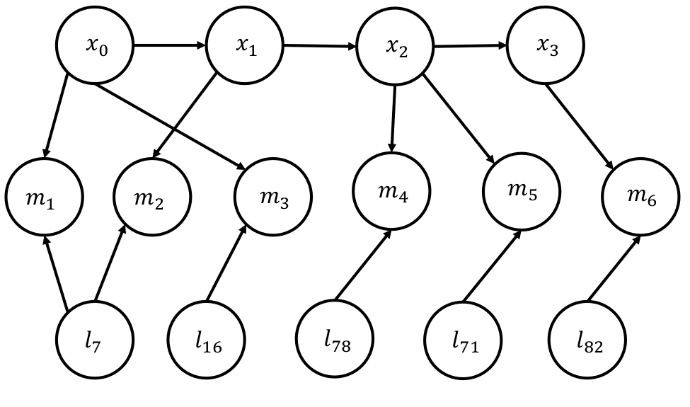
Because the Bayesian graph has no differentiation between known and unknown quantities for representation, the complexity of solving the graph is high even for a small number of parameters. As estimating the Maximum a-Posteriori (MAP) for just 3 measurements involes 6 factors and this grows exponentially making the process very very slow. We will not discuss how this is done as it is out of the scope of this class. Interested readers are referred to this article. A better representation model is a Factor Graph. In the factor graph model, only the unknown quantities are represented in nodes/bubbles. The known quantities and constraints are encoded in the solid squared and edges. This representation makes it super easy to understand the problem in hand. To do an MAP inference, we maximize the value of the graph which will be defined later mathematically. Let us first look at the factor graph image.

A Hidden Markov Model (HMM) represented as a Factor graph for the SLAM/SfM problem. Notice how easy the graph is to understand as compared to the Bayesian graph we saw before.

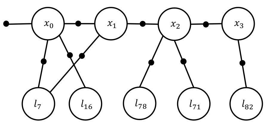
First, let’s talk about some factor graph terminology. A Unary factor is a factor which is connected only on one side to an unknown. This represents the prior information and is used to represent the initial state of the robot. For eg., look at the factor connected to \(\mathbf{x_0}\). Each contraint is associated with a covariance matrix which indicates how strongly one should enforce it for the optimization. Think of it as a measure of amount of slack you want to cut to that constraint in that particular optimization. If we really want to enforce the constraint that the initial pose is the origin, we would choose a very small covariance for it. A Binary factor is a factor which is connected on both sides to unknowns. This represents the constraints between the two unknowns. This is generally used to represent the measurements of the landmarks and the odometry. Note that the appripriate covariance needs to be used (\(\Sigma_m or \Sigma_o\)).

Now, let’s dive into the math which is working behind the mask of the factor graph.

Prior:

Here, \( \phi\) represents the value of the factor and \(P\) represents the probability function. Prior is represented using a unary factor.

Motion Model/Odometry:

Here, \(\mathbf{u_t}\) represents the control signal given to the robot to move from \(\mathbf{x_{t-1}}\) to \(\mathbf{x_t}\). Motion Model/Odometry is represented using a binary factor.

Measurement/Observation Model:

Here, \( \mathbf{m_{t,k}} \) is the measurement of \(k^{\text{th}}\) landmark \(\mathbf{l_k}\) at time \(t\). Measurement/Observation Model is represented using a binary factor.

The MAP problem/value of the graph to maximize is defined as follows:

Here, \(\mathbf{X}, \mathbf{L} \) represents the set of all states and landmark locations and \(T\) is the final time when the robot stops. GTSAM uses either a Levenberg Marquardt or the Dogleg optimizer to obtain the MAP estimates of the unknown parameters.

The code for the example in this toy example can be found on Nitin’s github here. Feel free to play around and ask any questions you have to the TAs.

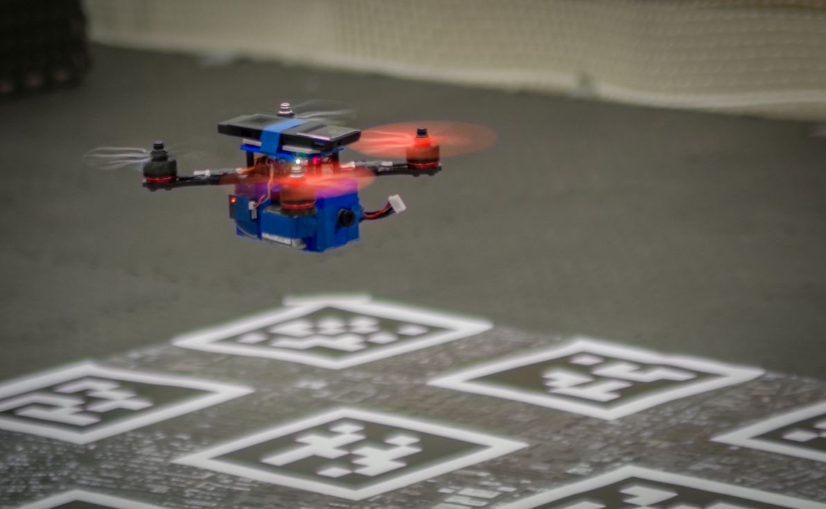
Now, that we’ve understood the Toy example (If you haven’t played around with Nitin’s code, now is a good time to do so!). Let us focus on the task in the project. The images for the project are taken from a quadrotor/drone flying over a carpet of april tags with New York’s cityscape (taken from Google Maps) in-between the tags for added features in-case you decided to get creative and use it for odometry. A photo of the data being collected is shown below:

A quadrotor flying over a carpet of April Tags. The quadrotor is equipped with a front facing camera, a downward facing camera and an Inertial Measurement Unit (IMU).

Now, let’s talk about what this “magical” April tag is. An AprilTag is a visual fiducial (something of a known shape and size) system, useful for a wide variety of tasks including augmented reality, robotics and camera calibration. It was developed by the April lab at the University of Michigan, Ann Arbor. It is one of the most common fiducial markers used in robotics. Though it is slow, it is extremely robust and works well for even a very small tag size. There have been better fiducial markers developed over the years, some of them are: ChromaTag, RuneTag and CCTag. Because of it’ robustness and commonality, we’ll use the AprilTag. Specifically we’ll use AprilTags v2 because of it’s higher speed as compared to AprilTags v1 with minimal loss in robustness.

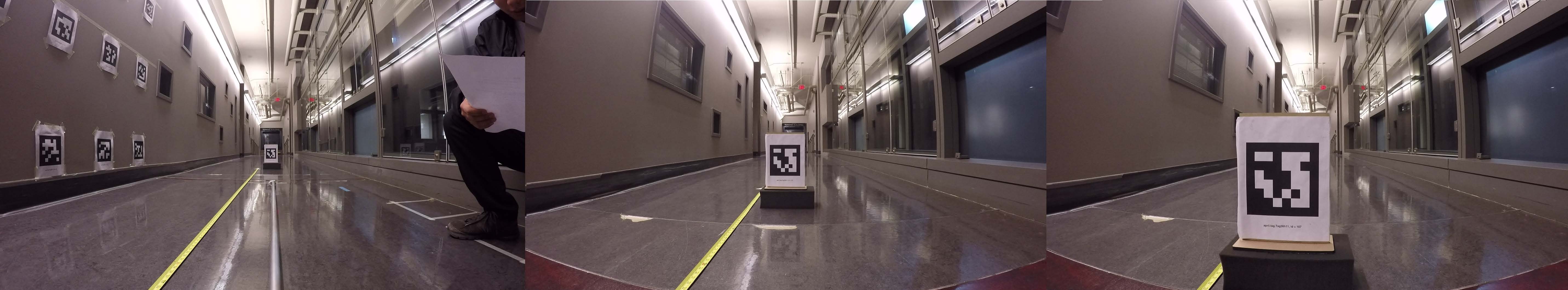
Let us consider the pose estimation of a camera given one AprilTag. The AprilTag library gives us the location of the tag corners on the image. Refer to Nitin’s Github for a link to the modified wrapper which can be run from Matlab directly using the system command. A sample of how an April Tag looks in the camera image is shown below:

How the AprilTag looks at different distances on the image.

The output of the April Tags library are shown are red, green, blue and magenta circles (the corners of the tags in the image).

Notice that we only obtain the tag corner locations on the image. We need to compute the camera pose from these corners. We have encoutered this scenario before, i.e., given the image coordinates \(\mathbf{x}\) and their corresponding world coordinates \(\mathbf{X}\), we need to compute the camera pose. This is exactly the same as the Perspective-n-Point problem we saw earlier. Let us consider a special case of this problem, if we assume that all the points lie on a plane (for the april tag it does anyway). The transformation from the world to the image plane becomes a Homography. Let us write this down mathematically. The projection formula is given by:

Here, \( R = \begin{bmatrix} r_1 & r_2 & r_3 \end{bmatrix}\) is the rotation matrix representing the orientation of the camera in the world and \(T\) is the translation or position of the camera in the world.

Because, we are interested in finding the pose of the camera \( \begin{bmatrix} r_1 & r_2 & r_3 & T \end{bmatrix} \) with respect to the april tag \(\mathbf{X}\), and we know that the april tag is on a plane. We can arbitraily chose the world coordinate as \(Z=0\), i.e., the tag’s plane in the world is the \(Z=0\) plane. This can be mathematically written as:

Now, let us denote \( \begin{bmatrix} r_1 & r_2 & T \end{bmatrix} \) as \( H \), the homography matrix which encompasses the pose of the camera. We are intersted in finding the pose of the camera, i.e., \( R, T\).

We need a minimum of 4 point correspondences between the tag image locations and the world points to uniquely determine the pose of the camera. Luckily, we have 4 corners in the April Tag. Now the rotation matrix which can be formed from the values of \(K^{-1}H \) are given by \( \begin{bmatrix}h_1’ & h_2’ & h_1’ \times h_2’ \end{bmatrix} \). However note that, this only guarentees that the columns are orthogonal but not that the determinant as +1, i.e., this solution doesn’t guarentee a valid rotation matrix. The optimization problem is to find a valid rotation matrix closest to the solution we found in the last step. This can be mathematically written as:

Where the norm used in the above equation is called Frobenious Norm.

As always, our best friend SVD can help us solve the above optimization problem.

The “best” valid rotation matrix approximating the above matrix is given by:

The diagonal matrix ensures/improses the constraint that the determinant is +1 and because U, V^T are obtained from the decomposition of \( \begin{bmatrix}h_1’ & h_2’ & h_1’ \times h_2’ \end{bmatrix} \), the orthonomlaity is automatically satisfied. Hence \(R\) is a valid rotation matrix.

The translation/position can be found as:

However, in the most general case one would need to stick to solving the PnP problem.

The project you are solving is closely related to Nitin’s Masters Thesis at the University of Pennsylvania. The concepts used in the Thesis are also presented in Nitin’s ICRA paper. More details about the project can also be found on the PennCOSYVIO’s project website.

Now, that we have all the ideas we need to tackle the problem in hand, let us remind ourselves of the problem in hand. We are given data from a downward facing camera of a quadrotor flying over a carpet of april tags. We want to estimate the pose of the camera/quadrotor at every-time instant whilst localizing the april tags in the “chosen” world reference frame. This problem of camera pose estimation is very easy if the locations of the tags in the world is known and this merely reduces to a Homography estimation problem in case of planar tag placement or PnP in general. However, generally we don’t know the locations of the tags in the world. In such cases, we need to simultaneously estimate the pose of the camera and the locations of the tags. This is called Structure from Motion (SfM) or Simultaneous Localization and Mapping (SLAM).

Now, let us collate all the information we know about the scene.

• The carpet of april tags are placed over the floor which can be assumed to be a flat surface/plane.
• The quadrotor is moving reasonably slowly.
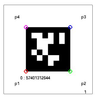
• Let us choose the first tag detection in the first frame as the world origin and the vector in the direction of \(p_1\) to \(p_2\) be world \(X\) and vector in direction of \(p_1\) to \(p_4\) be world \(Y\). Refer to figure below.
• All april tags are of the same size and this size is known.
• The april tags are rigidly attached to the ground with minimal effect from the downforce of the propellers of the quadrotor.

The output of the April Tags library are shown are red, green, blue and magenta circles (the corners of the tags in the image).

Now, we can start building the Factor Graph for the Bundle Adjustment part in the SfM/SLAM pipeline.

• The initial pose of the camera can be estimated from just one tag (first detection which we chose as the origin) using Homography. This constraint is added to the factor graph as a PriorFactor.
• The world coordinates of the first tag detected is chosen as the origin and this constraint is added to the factor graph as a PriorFactor as well.
• The relative poses between the camera at consecutive times \( t\) and \(t+1\) are very close as the camera is not moving fast. Hence a BetweenPointFactor constraint with Identity transformation can be used in the factor graph.
• The projection of the world coordinates onto the image coordinates is fed into the factor graph using a GenericProjectionFactor.
• The size of the tags in the world is known and is fixed. This constraint is fed into the factor graph using a BetweenFactor between the world locations of a particular april tag.

Note that each factor in the factor graph is modelled with a gaussian noise model, i.e., the flex in the constraints of the graph are represented by a covariance matrix. The values of these covariance matrix represent the amount of trust in that particular constraint. For eg., we chose the origin so we want to enforce that constraint tightly, so the covariance might say that, I allow only 1mm of flex in this constraint to account for some measurement errors. However, the constraint that we didnt move much between time instants can be a little more relaxed and we might say that we allow it to flex by 3cm between frames and so on. The initial values are given by the pose estimated from Homography and so on.

This resulting factor graph is shown below:

The factor graph for Bundle Adjustment in SfM/SLAM problem. \(\mathbf{x_t}\) represents camera pose at time \(t\) and \(\mathbf{L_k^i}\) represents the \(i^{\text{th}}\) corner of the \(k^{\text{th}}\) tag. We want to estimate the things in the bubble and the solid/filled bubbles are the constraints imposed. The constraints for the 100\(\text{th}\) landmark and \(x_1\) are not shown for the purpose of brevity.

One could use the LevenbergMarquardtOptimizer or the DoglegOptimizer to solve for the parameters of the graph.

Detailed Explanation of Project 4

Now, let’s look at how GTSAM will be used in Project 4. As mentioned in the project desciption, we are given detected april tag corners in the frames of a video sequence. We want to find the 3D locations of these april tag corners in the world frame and the pose (position and orientation) of the camera in the world frame for every video frame. Now, let’s recall all the information we know in this project.

• The carpet of april tags are placed over the floor which can be assumed to be a flat surface/plane.
• The quadrotor is moving reasonably slowly.
• Let us choose the first tag detection in the first frame as the world origin and the vector in the direction of \(p_1\) to \(p_2\) be world \(X\) and vector in direction of \(p_1\) to \(p_4\) be world \(Y\).
• All april tags are of the same size and this size is known.
• The april tags are rigidly attached to the ground with minimal effect from the downforce of the propellers of the quadrotor.

In order for GTSAM to work well, we need to initialize the values of the factor graph to a reasonable values. The next part of this section talks about building the factor graph and initializing the values.

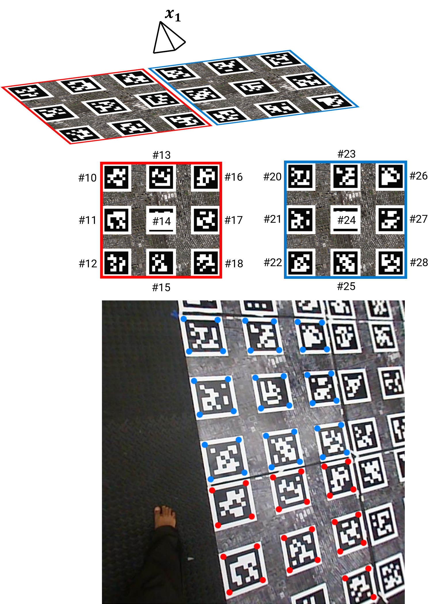
Let us consider the first frame of a sequence. Let us denote the pose of the camera as \(x_0\) and let Tag 10’s left bottom corner be the world origin as shown in the Figure below. Here the X-Y-Z axes are shown in Red, Green and Blue respectively. A top view of the world is shown in the top right hand side of the figure with the Tag ID’s (10 to 18) highlighted.

The camera pose in the first frame is \(x_0\). Bottom row shows the image seen by the camera (video frame) with detected april tag corners highlighted in red.

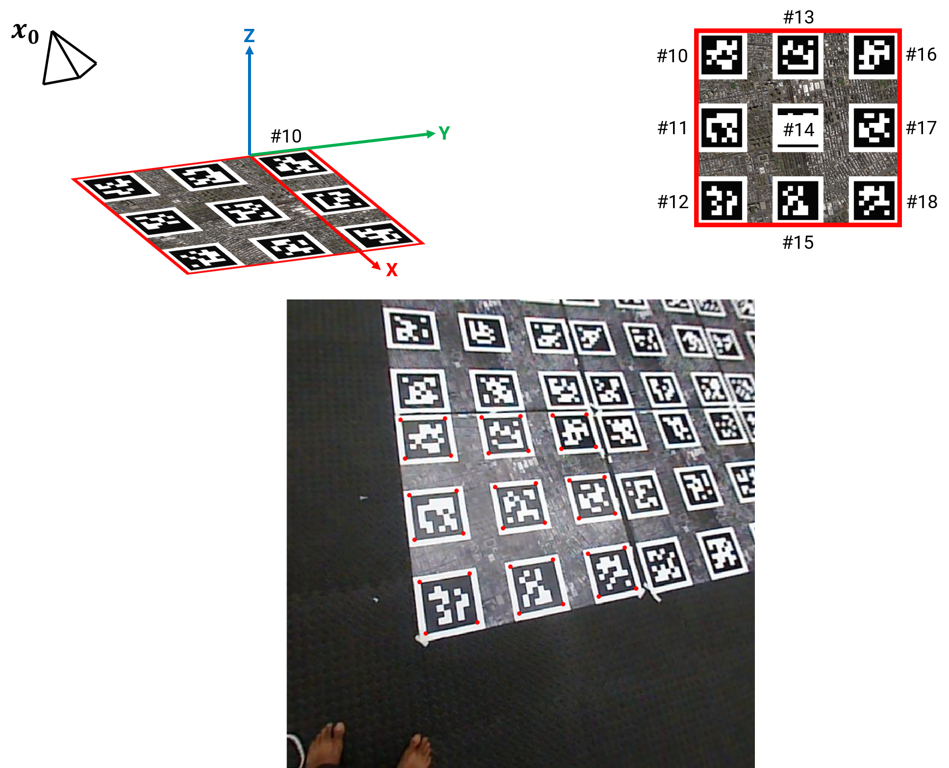
Also, observe the video frame/image in the bottom row with detected tag corners highlighted in red. The data given to us are these detected tag corners (the ones shown as red dots). Now, let’s look at the factor graph corresponding to the first frame. We need to initialize the values in the bubble and specify the contraints denoted by the solid bubbles. First of all, Tag 10’s left bottom corner was chosen as the origin, this can be fed as a PriorFactor on the \(L_{10}^1\). Now, we want to obtain a value for the initial pose \(x_0\). This can be done by the knowledge of the pose of any (one or more) tags. Note that, until now, we only know the pose of Tag 10 (as we chose it as the world origin). To estimate \(x_0\) given \(L_{10}^1, L_{10}^2, L_{10}^3, L_{10}^4\), we’ll use the homography equations we discussed before (because both the tag in the world and in the image are planar in nature). Using these homography equations, we obtain the pose of the camera with respect to the Tag 10 World frame, i.e., \(R_0\) and \(T_0\) which together constitute the value of \(x_0\).

Factor Graph for Frame 1. The things in the bubble need to be initialized, the the solid bubbles are constraints. Things in code font (courier font) refer to the GTSAM syntax and normal font refer to explanations.

Now, we need to initialize the world frame co-ordinates of other tags (other than Tag 10, 11-18 in this example). Recall that we have the pose of the camera \(x_0\) in the world frame and the image co-ordinates of the tag corners. To obtain the world frame co-ordinates of other tags it is as easy as plugging in the values to the camera projection equation or the pinhole model.

Here, we need to obtain the values of \(\begin{bmatrix} X \ Y \ Z \ W \end{bmatrix}^T\) given other values in the equation.

Now, let’s look at the second frame as shown below.

The camera pose in the second frame is \(x_1\). Middle row shows the top view of the world frame with Tag IDs. Bottom row shows the image seen by the camera (video frame) with detected april tag corners highlighted in red and blue. The red tag corners denote the tags common between frames 1 and 2 and blue tag corners denote the new tags observed in frame 2 which were not seen in frame 1.

The graph for this frame is shown below.

Factor Graph for Frame 2. The things in the bubble need to be initialized, the the solid bubbles are constraints. Things in code font (courier font) refer to the GTSAM syntax and normal font refer to explanations.

As before, we need to initialize the pose of the camera \(x_1\) given the knowledge of the pose of any (one or more) tags. Now, we have knowledge of the pose of all the common tags we saw in both frames 1 and 2 (red corners in frame 2’s image). We can use the homography equation again to obtain the value of \(x_1\) (Note that here we have a lot more than 4 equations in contrast to frame 1).

To obtain the world frame co-ordinates of blue corners (\(L_{18}^1 \cdots L_{28}^4 \)) we use the pinhole equation as before given the pose of the camera \(x_1\) and the image co-ordinates of these tags.

However, we moved from \(x_0\) to \(x_1\) as shown below.

The camera moved from \(x_0\) in frame 1 to \(x_1\) in frame 2.

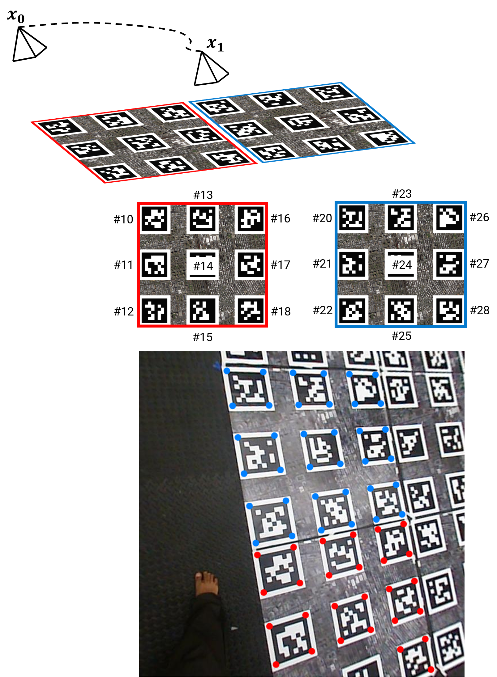
If we add in the constraint between the two camera poses, we obtain the factor graph given below.

Factor Graph for frames 1 and 2.

The BetweenFactor between \(x_0\) and \(x_1\) indicates an odometry measurement obtained from different source such as an IMU. Since we made the assumption of slow movement, we’ll add an identity value for this constraint.

For debugging this project, we would recommend plotting the world tag corner locations and camera poses without factor graph optimization (by using the values which will be used to initialize) first. It should look sensible but not perfect.

When these values are plotted, notice that the drift (deviation of corners from their actual locations) accumulates over time (as frame number increases). This is sometimes the issue when such values are fed into GTSAM. One simple way (not optimal in any sense) to solve the problem is by first running GTSAM in small batches of frames and reusing these values for the final GTSAM graph.

Hope you loved this assignment. As a parting thought, these methods are used in today’s self driving cars to make a map of the world in real-time. However, they are also fused with deep learning based methods to speed up the computation. Have a look at this video for a cool behind the scenes look of the NVIDIA’s self driving platform.